Controlling the Distance of the robot from a Target

GTA Marking

This is an assessed Exercise. When you have completed the Assessed Exercise, you should show your work to a GTA to get marked.

Before Continuing

Before starting these exercises, you should ensure that you have completed all the Basic Exercises and have fully constructed the robot chassis, as described in the Building the Robot document.

Introduction

In this exercise, you will implement a closed-loop distance control system designed to maintain a fixed offset between the robot chassis and a moving target. The system uses a Proportional-Integral (PI) controller, an infrared (IR) distance sensor for distance feedback, and PWM actuation signals routed to the motor driver board (TB6612FNG).

The schematic and breadboard wiring requirements for this task are identical to those defined in the Motor and Encoder Exercise.

The following video demonstrates the closed-loop tracking response of the completed system:

Video demonstrating the expected outcome from this exercise

The PI Controller Algorithm

The theoretical principles of Proportional-Integral (PI) control is covered in your course notes from other modules, and therefore, will not be comprehensively covered in this section.

A PI controller adjusts system behaviour, in this case, maintaining the relative distance between the robot chassis and a target object. The PI algorithm operates inside a closed-loop feedback structure, as illustrated in the block diagram below:

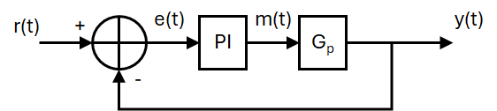
Block diagram of the closed loop control system, showing the PI controller.

Where: $R(t)$ is the reference signal, $e(t)$ is the error signal, $m(t)$ is the manipulated variable and $y(t)$ is the system output, and $Gp$ is the process dynamics of the robot chassis.

The structure of the PI controller is shown above, and can be represented with the following time domain equation:

\[ m(t) = \underbrace{K_p\,e(t)}_{\text{Proportional Term, }p(t)}+\space\space\space\space\space\space\overbrace{K_i\int_{-\infty}^\infty e(t)\,dt}^{\text{Integral Term ,}i(t)} \, \]

A Block diagram of the above PI controller algorithm is shown below:

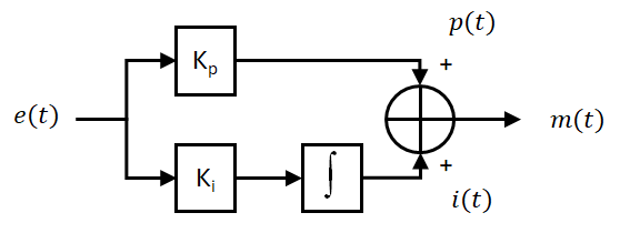
Block diagram representation of the PI controller.

Where: $e(t)$ is the error, $p(t)$ is the proportional term, $i(t)$ is the integral term, and $m(t)$ is the manipulated variable. $K_p$ and $K_i$ are the controller gains.

The continuous-time PI controller algorithm cannot be directly executed on a digital microcontroller like the ATmega328P; it must first be discretized into a discrete-time difference equation.

To achieve this, split the controller output into separate proportional, $p(t)$, and integral, $i(t)$, terms, then discretize each component individually:

The proportional term: $ p(t)=K_p\,e(t)=K_p(r(t)-y(t)) $
- This discretizes to: $ p[k]=K_p\,e[k]=K_p(r[k]-y[k]) $, where: $k$ is the current time step.
The integral term: $i(t)=K_i\int_{-\infty}^\infty e(t)\,dt \space\space \Longleftrightarrow \space\space \frac{di(t)}{dt}=K_i\,e(t) $
- We can use a Backward difference method, to discretize the derivitive function:
\[ \frac{di(t)}{dt}=K_i\,e(t) \space\space \Longleftrightarrow \space\space \frac{i[k]-i[k-1]}{\Delta T}=K_i\,e[n] \space\space \Longleftrightarrow \\ \space\space i[k] = i[k-1]+K_i\,e[n]\,\Delta T \]

Where: $\Delta T$ is the sample period for the controller.
Finally, the manipulated variable, $m[k]$, can be found:

\[ m[k] = p[k] + i[k] = K_p \, e[k] + i[k-1] + K_i \, e[k] \, \Delta T \]

Integral Anti-Windup Protection

The integral term is susceptible to integral wind-up—a condition where persistent error causes the accumulated integral term to grow excessively beyond the physical actuation capability of the system.

To mitigate wind-up during large steps or saturated conditions, clamp the integral term ($i[k]$) within bounds corresponding to the maximum allowable PWM output range (i.e., $\pm 255$ for the PWM implementation we are using):

Integral Term Saturation

if (i > 255.0) {
    i = 255.0;
} else if (i < -255.0) {
    i = -255.0;
}

where i is the floating-point variable storing the discrete integral state, $i[k]$.

To maintain modularity and keep the main loop() concise, the discrete PI controller algorithm should be encapsulated inside a dedicated function, as demonstrated below:

Example code for a PI controller function

int piControllerfunction(float contrKp, float contrKi,
        float contrRef, float contrFB, float deltaT){

    // Calculate the control error
    contrError = contrRef - contrFB;

    // Calculate the proportional term
    float p = contrError * contrKp

    // Calculate the integral term
    float i = iPrev + (contrError * contrKi * deltaT)

    // Bound the integral term to 255
    if i > 255 {
        i = 255;
    }
    else if (i < -255) {
        i = -255;
    }

    // calculate the manipulated variable
    float m = p + i

    // Bound the manipulated variable to 255
    if m > 255 {
        m = 255;
    }
    else if (m < -255) {
        m = -255;
    }

    // Save the integral term for the next iteration
    iPrev = i;

    // Recast the manipulated variable and return its value
    return (int)m;
}

Implementation Details for calculatePI()

Periodic Execution: The calculatePI() function must be called at a fixed, deterministic sampling interval within the main() execution loop. In our example implementation, shown in Fig 1, a sample period of $\Delta T = 10\,\text{ms}$ ($100\,\text{Hz}$) was used.
Persistent Integral State: The variable storing the previous integral accumulator (iPrev) must persist across function calls. Declare and initialize it in global scope.
Function Parameters: The controller parameters—proportional gain (contrKp), integral gain (contrKi), reference setpoint (contrRef), sensor feedback (contrFB), and sample period (deltaT), must be passed as floating-point arguments to the function.

A Note on Code Timing and Determinacy for Embedded Systems

When implementing a digital PI controller on an embedded microcontroller, maintaining strict, deterministic execution timing is critical. Sensor readings, error evaluation, and discrete integration must occur at precise, fixed time intervals ($\Delta T$). Unintended variations in sampling interval (sampling jitter) degrade control accuracy and can destabilize the feedback loop.

Using blocking delay functions like delay() creates inconsistent timing and prevents concurrent task execution. Because code execution time varies depending on conditional logic and system state, blocking delays make deterministic sampling nearly impossible to maintain.

To enforce consistent timing, use non-blocking scheduling based on the millisecond timer function millis(), as demonstrated in the TwoInterruptEncoder.ino example. In that example, non-blocking timing controls periodic Serial Monitor telemetry printing within the main execution loop (loop()).

Assessed Exercise

In this exercise, you will write a program to maintain a fixed distance between the robot chassis and a target object. You will implement a closed-loop control system using a Proportional-Integral (PI) controller, an infrared (IR) sensor for distance feedback, and PWM actuation signals routed to the motor driver board (TB6612FNG).

Procedure:

Ensure that you have the completed the building of the robot chassis and the electronic circuit, as described in the Building the Robot Chassis document.
A good starting point for the code for this exercise is the assessed exercise you completed for the Motor and Encoder section
The lolly stick should be raised to the vertical position at the start of the exercise demonstration.
Write a program that maintains the robot chassis 30cm from a target, (the kit box stood up on its end works well for this):
1. Uses the IR sensor to measure the distance to the target
2. The robot chassis should be actuated using the yellow gear motor, with wheel attached, and driven from the driver board.
3. A PI controller must be used to control the system in closed loop, with the output of the PI controller providing the PWM signal, and setting the BI1 and BI2 inputs to the driver board.
4. The following controller gains should be used:
  - $K_p = -10$
  - $K_i = -20$
Ensure the code you write does not use the delay() function to control timing in the main function, loop(), instead use the millisecond tick timer function, millis(), to provide a timing source for your code execution.
- In our example implementation, shown in Fig 1, we used a control sample period of $\Delta T = 10\,\text{ms}$.

Note

The $K_p$ and $K_i$ values are negative because of the negative slope of the IR sensor response.

The controller values have been selected to show a slight overshoot when the target is moved, if used with a control sample period of 10ms.

Exercise Assessment

What we expect to see from your demonstration?

At the start of the demonstration, your robot chassis should be placed approximately 30cm from the target, (the kit box stood up on its end works well for this).
On resetting the Arduino, your lolly stick should go to the horizontal position, if it is not already there.
After a one-second delay, the lolly stick assembly should raise to the vertical position.
After a further one-second delay, the robot chassis should start to track the position of the target.
You must show that you have implemented the position control using a PI controller.

Now Get Your Work Marked by a GTA

Once you have completed your code and are satisfied with its operation, you should show your work to a GTA for marking.